How Diffusion Models Work — Building Stable Diffusion From Scratch (Part 2)

This is not a "text-to-image in 5 minutes" post.
This is not hype.
This is the actual math and code behind modern generative AI.

If Part 1 taught you how neural networks learn, this post teaches you how modern image generators exist at all.

### Table of Contents

1. What Is a Diffusion Model, Really?
2. The Forward Diffusion Process (Adding Noise)
3. The Noise Schedule (Why It Matters)
4. Sampling Noisy Images at Any Timestep
5. What the Model Is Trained to Predict
6. The UNet Architecture
7. Loss Function and Training Objective
8. The Training Loop
9. Reverse Diffusion (Image Generation)
10. Why Diffusion Models Actually Work
11. Final Thoughts

### What Is a Diffusion Model, Really?

A diffusion model does not generate images directly.

Instead, it learns one very specific skill:

Given a noisy image, predict the noise that was added to it.

That’s it.

If you can do that reliably at every noise level, you can:

• start from pure noise
• repeatedly remove noise
• end up with a realistic image

This idea is borrowed from statistical physics and probability theory, not biology.

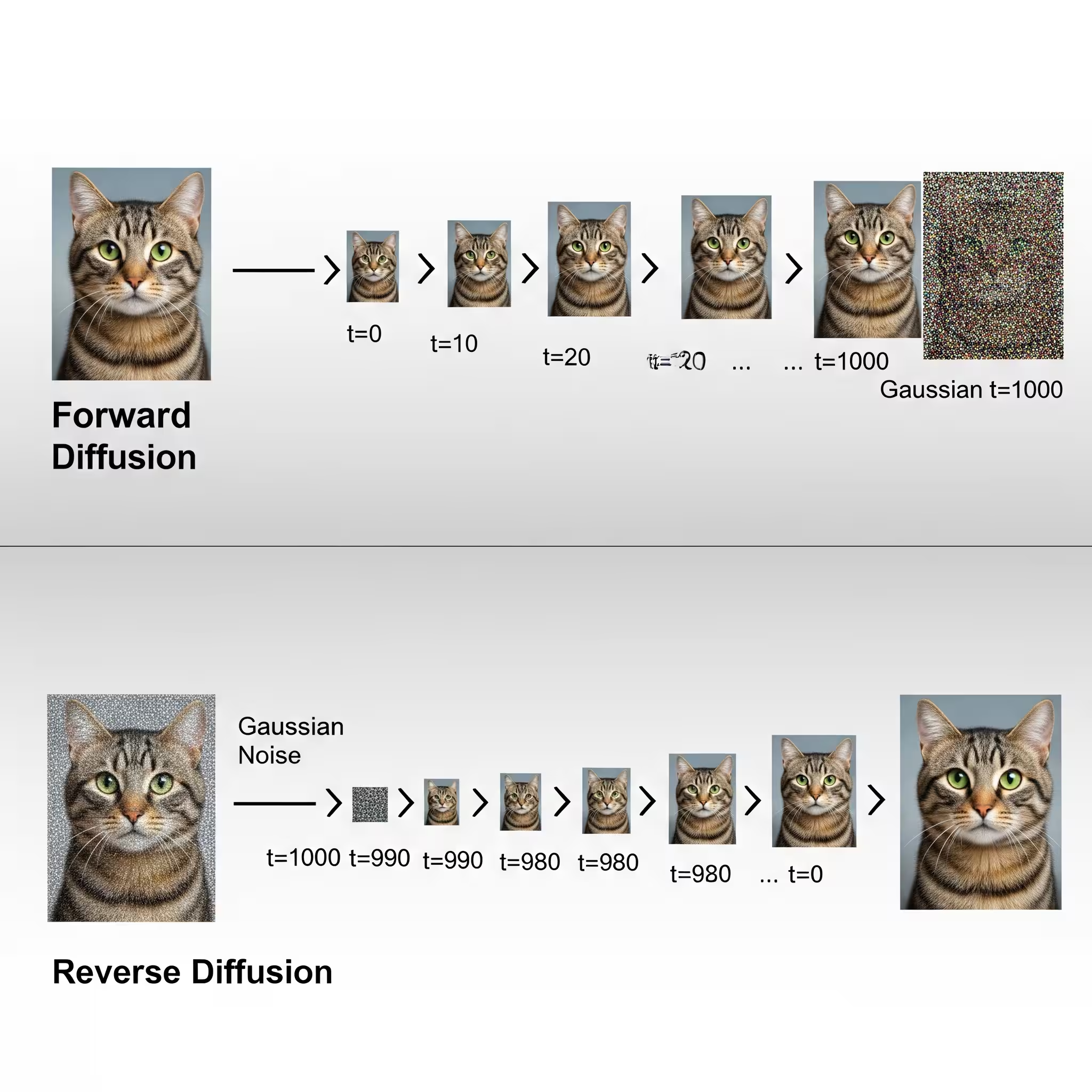
### The Forward Diffusion Process (Adding Noise)

The forward process slowly destroys information.

At timestep (t = 0), the image is clean.
At timestep (t = T), the image is pure Gaussian noise.

This happens gradually to avoid destroying structure too quickly.

### The Noise Schedule (Why It Matters)

We control how much noise is added at each step using a beta schedule.

import torch

def linear_beta_schedule(timesteps):
    beta_start = 0.0001
    beta_end = 0.02
    return torch.linspace(beta_start, beta_end, timesteps)

#### Explanation

• beta controls noise variance per step
• Small values preserve structure early
• Larger values ensure complete destruction later
• Linear schedules are simple and stable for learning

More advanced models use cosine schedules, but the concept is identical.

### Sampling Noisy Images at Any Timestep

Instead of adding noise step-by-step, diffusion uses a closed-form equation:

[
x_t = \sqrt{\bar{\alpha}_t} x_0 + \sqrt{1 - \bar{\alpha}_t} \epsilon
]

This allows direct sampling at any timestep.

def q_sample(x_start, t, noise=None):
    if noise is None:
        noise = torch.randn_like(x_start)

    sqrt_alpha_hat = torch.sqrt(alphas_cumprod[t])[:, None, None, None]
    sqrt_one_minus = torch.sqrt(1 - alphas_cumprod[t])[:, None, None, None]

    return sqrt_alpha_hat * x_start + sqrt_one_minus * noise

#### Explanation

• x_start is the clean image
• noise is Gaussian noise
• The model sees all corruption levels, not just extreme cases

This single equation makes diffusion computationally practical.

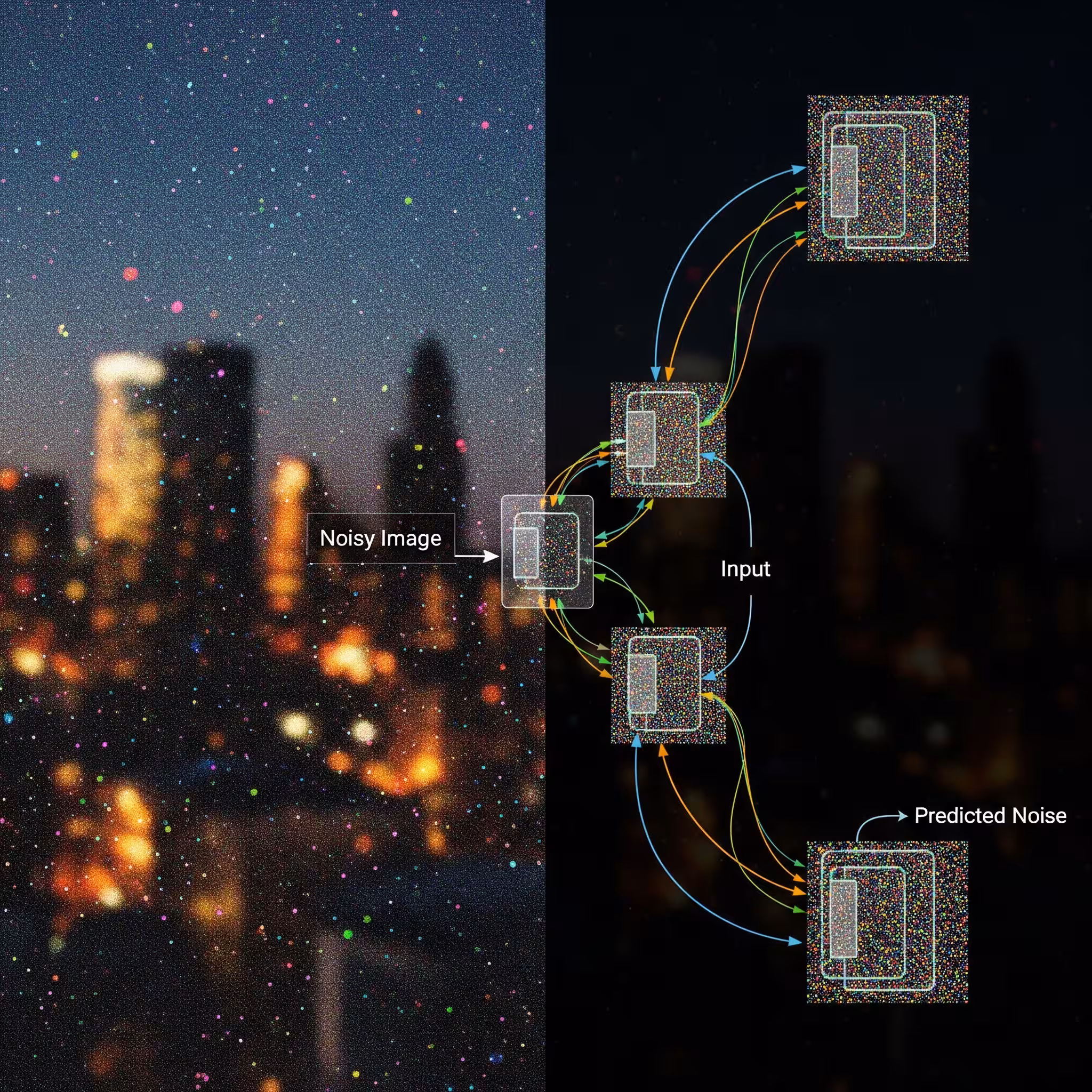
### What the Model Is Trained to Predict

The model does not predict images.

It predicts:

[
\epsilon_\theta(x_t, t)
]

Which means:

The noise that produced the current image.

Predicting noise instead of pixels:

• stabilizes training
• avoids blurry outputs
• aligns with maximum likelihood estimation

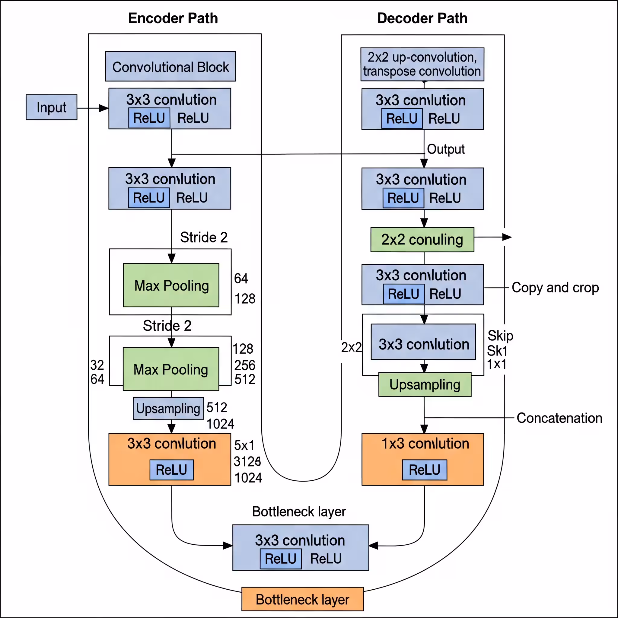
### The UNet Architecture

Diffusion models use UNets because they:

• preserve spatial information
• capture global context
• reconstruct fine details

import torch.nn as nn

class SimpleUNet(nn.Module):
    def __init__(self):
        super().__init__()

        self.down1 = nn.Sequential(
            nn.Conv2d(3, 64, 3, padding=1),
            nn.ReLU()
        )

        self.down2 = nn.Sequential(
            nn.Conv2d(64, 128, 3, padding=1),
            nn.ReLU()
        )

        self.up1 = nn.Sequential(
            nn.ConvTranspose2d(128, 64, 3, padding=1),
            nn.ReLU()
        )

        self.out = nn.Conv2d(64, 3, 1)

    def forward(self, x):
        d1 = self.down1(x)
        d2 = self.down2(d1)
        u1 = self.up1(d2)
        return self.out(u1)

This minimal UNet is enough to understand diffusion deeply.

### Loss Function and Training Objective

The training objective is simple:

def diffusion_loss(model, x_start, t):
    noise = torch.randn_like(x_start)
    x_noisy = q_sample(x_start, t, noise)
    noise_pred = model(x_noisy)
    return nn.MSELoss()(noise_pred, noise)

#### Why MSE?

• Noise is Gaussian
• MSE corresponds to maximum likelihood
• Predicting noise avoids instability

The model learns to reverse corruption — not to hallucinate images.

### The Training Loop

optimizer = torch.optim.Adam(model.parameters(), lr=1e-4)

for epoch in range(epochs):
    for images in dataloader:
        t = torch.randint(0, timesteps, (images.size(0),))
        loss = diffusion_loss(model, images, t)

        optimizer.zero_grad()
        loss.backward()
        optimizer.step()

    print(f"Epoch {epoch} | Loss: {loss.item()}")

#### What This Teaches the Model

• All noise levels are learned
• No discriminator needed
• Training is slow but stable

This stability is why diffusion replaced GANs.

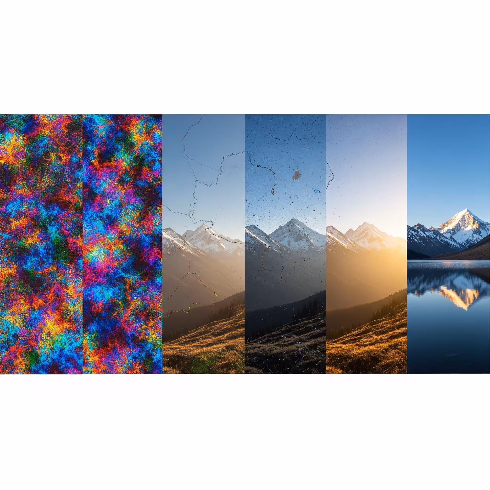
### Reverse Diffusion (Image Generation)

Image generation is the reverse of noise addition.

@torch.no_grad()
def sample(model, shape):
    x = torch.randn(shape)

    for t in reversed(range(timesteps)):
        noise_pred = model(x)

        alpha = alphas[t]
        alpha_hat = alphas_cumprod[t]
        beta = betas[t]

        x = (1 / torch.sqrt(alpha)) * (
            x - ((1 - alpha) / torch.sqrt(1 - alpha_hat)) * noise_pred
        )

        if t > 0:
            x += torch.sqrt(beta) * torch.randn_like(x)

    return x

This loop slowly reveals structure from randomness.

### Why Diffusion Models Actually Work

Diffusion models succeed because they:

• model the full data distribution
• avoid adversarial instability
• reduce generation to denoising

They trade speed for reliability.

### Final Thoughts

Diffusion models are not magic.
They are patience, math, and repetition.

If you understand this post, you understand the foundation of:

• Stable Diffusion
• DALL·E
• Imagen

This is Part 2.

Next comes conditioning, latent diffusion, and real-world scaling.